The Term Structure of Cross Correlations between the Kerosene and Crude Oil Markets
Are correlations across assets constant for every time interval?
Let´s analyze this question taking two series in the energy sector: kerosene and crude oil prices.
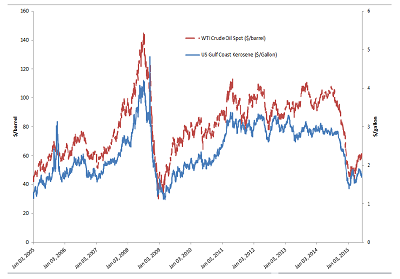
Fig 1

Fig 1 graphs the time evolution of the daily spot price of WTI crude oil in US $/barrel (dashed line) and for jet kerosene in $/gallons (solid line) from January 2005 to June 2015. The data source is the US Energy Information Administration (EIA) which provides data for both series using the two reported measures, for which we use two different axes, ($/barrel on the left $/gallon on the right). The picture reflects two important features:
a) the two series are nonstationary (meaning that they exhibit different distributions across time)
b) there is a clear comovementin their price behavior.
This information is relevant for commercials such as kerosene hedgers. For instance, an airline company needs to protect itself against adverse movements in jet fuel prices. Since jet fuel futures markets are not liquid, the airline uses crude oil futures to hedge its price risk. The efficiency of this approach is determined by the extent which the series commove during the time interval of the price exposure.
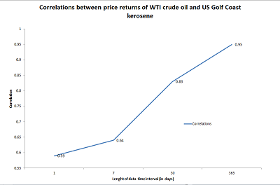
The correlation between price changes is a crucial determinant of the optimal hedging strategy for a cross hedge. The common approach in the literature is to obtain the optimal hedge ratio by using the most frequent returns available, irrespective of the time to maturity. This approach will always work if the correlations between price returns are constant with respect to the sampling frequency as it is the case under two correlated Brownian Motions. However, as stated in Ankirchner et al. (2012) it is commonly observed that correlations between financial assets are strongly determined by the time interval. If we look at Fig 2 which depicts the correlation coefficient for four different data intervals: 1 day, one week (7 days), one month (30 days) and 1 year (365 days) we can see that there is an increasing term structure of the correlation structure between both series. In fact, the correlation for daily price returns between kerosene and crude oil over our sample period is 0.59, which is weak given the strong co‐movement between the price series. However, correlations increase with the data frequency as demonstrated by the data figures corresponding to weekly, monthly and yearly correlation of returns which are 0.64, 0.83 and 0.95 respectively.
Fig 2

The observed increasing term structure of correlations between crude oil and kerosene returns shows that, as the frequency of the data is increased the two series become more synchronized in their movements. This suggests that there is a long term relationship between the two series with temporary deviations that are expected to be reflected in the higher frequency data. This feature is closely related to property of cointegration (see Engle and Granger 1987). Two non‐stationary series are cointegrated if there is a linear combination between them that is stationary or mean reverting. As opposed to the property of correlation the implication of cointegration is that two cointegrated price series cannot move in opposite directions for long periods without coming back to the long run equilibrium.
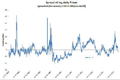
Fig 3 plots the error term (or log spread) resulting from a linear regression between kerosene and crude oil log prices. The behavior of the spread shows a clear mean reverting behavior. This property is formally tested using an Augmented Dickey Fuller on the log spread series.
Test results (available upon request) show that null hypothesis of non‐stationarity is rejected at the 1% significance level and that this property holds for every time interval considered (daily, weekly, monthly and yearly).
Fig 3

Data source EIA
Two interesting features can be drawn from the analysis:
When the two financial variables are cointegrated the order of cointegration holds irrespective of the selected time interval of the data, while the degree of correlation is expected to increase with the dating frequency.
This has important implications for the selection of optimal cross hedges. The optimal strategy will have to consider time varying hedge ratios that require adjustments in the hedging position in continuous time. Ankirchner et al. (2012) offer a close form solution to this problem taking into account the existence of a stationary spread of cointegrated time series. As stated in their paper “it is better to allow for a long term relationship rather than neglect it”.
Ankirchner, S., Dimitroff G., G. Heyne and C. Pigorch (2012). Futures “Cross‐Hedging with a Stationary Basis.” Journal of Financial and Quantitative Analysis, 47, 1361‐1395.
Engle, R.F., and C.W.J. Granger (1987). “Cointegration and error correction: Representation, estimation, and testing.” Econometrica, 55, 251‐276.


 Facebook
 Linkedin
 Instagram
 Youtube
 EMC Newsletter


